Binomial Trend Detection

The binomial trend detection method offers an alternative to traditional rolling averages by using week-over-week (WoW) comparisons to detect significant changes quickly.

Methodology

This approach involves:

• Calculating Week-over-Week Deltas: Measuring daily changes.
• Using a 14-Day Rolling Window: Smoothing out short-term fluctuations.
• Counting Positive and Negative Changes: Tallying the days with consistent directional shifts.
• Applying Statistical Analysis: Using the binomial distribution (for example, requiring 12 out of 14 days to exhibit the same trend) to confirm significant changes.

Process Details

Step	Details
Calculate WoW Deltas	Determine the day-to-day changes in the metric.
Rolling 14-Day Window	Apply a two-week window to balance sensitivity and stability.
Count Positive/Negative Days	Tally days with consistent positive or negative changes.
Binomial Distribution	Model the data with an assumption of a 50% chance for each day’s outcome.
Trend Threshold	Flag a trend if the count meets a predefined threshold (e.g., 12 out of 14 days).

binom.test(12, 14, 1/2, alternative = "greater")

    Exact binomial test

data:  12 and 14
number of successes = 12, number of trials = 14, p-value = 0.00647
alternative hypothesis: true probability of success is greater than 0.5
95 percent confidence interval:
 0.6146103 1.0000000
sample estimates:
probability of success 
             0.8571429 

library(ggplot2)
library(showtext)
library(ggtext)

showtext_auto()
showtext_opts(dpi = 300)

font_add_google(name = "Roboto", family = "Roboto")
font_1 <- "Roboto"

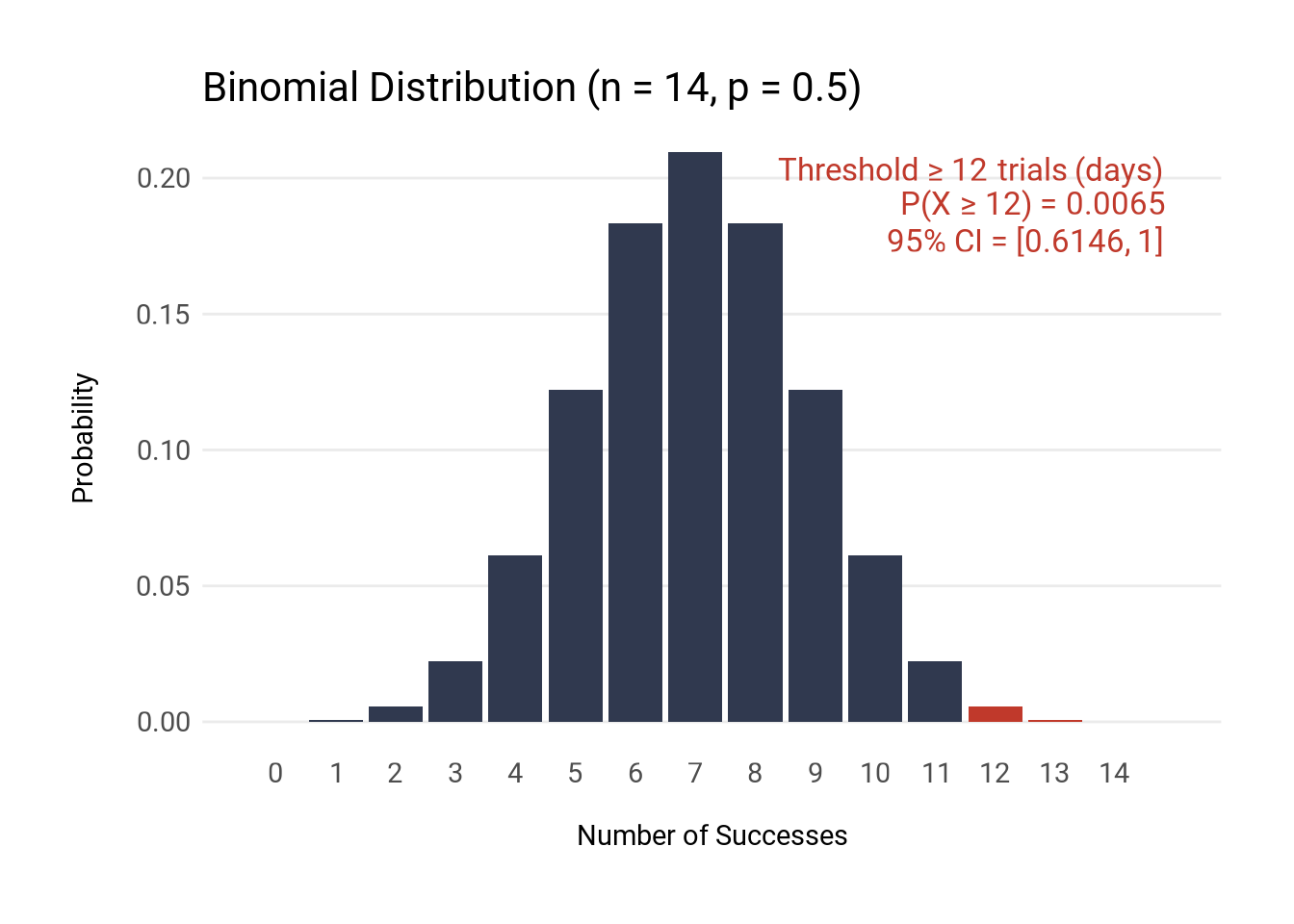
n <- 14 
p <- 1/2  
x_obs <- 12  

binom_test <- binom.test(x_obs, n, p, alternative = "greater")

p_value <- binom_test$p.value
conf_int <- binom_test$conf.int

p_ge_x_obs <- sum(dbinom(x_obs:n, size = n, prob = p))

data <- data.frame(
  x = 0:n,
  probability = dbinom(0:n, size = n, prob = p),
  color = ifelse(0:n >= x_obs, "#C0392B", "#30394F")  
)

binom_visual <- ggplot(data, aes(x = x, y = probability, fill = color)) +
  geom_bar(stat = "identity") +
  scale_fill_identity() +  
  scale_x_continuous(breaks = 0:n) +  
  labs(
    title = "Binomial Distribution (n = 14, p = 0.5)",
    x = "Number of Successes",
    y = "Probability"
  ) +
  theme_minimal() +
  theme(
    panel.grid.major.x = element_blank(),
    panel.grid.minor = element_blank(),
    plot.margin = margin(10, 10, 10, 10, "mm"),
    axis.text = element_text(family = font_1, size = 7),
    axis.title = element_text(family = font_1, size = 7),
    axis.title.x = element_text(margin = margin(5, 0, 0, 0, 'mm')),
    axis.title.y = element_text(margin = margin(0, 5, 0, 0, 'mm')),
    plot.title = element_text(family = font_1, size = 10)
  ) +
  annotate(
    geom = 'richtext',
    x = n+1,
    y = max(data$probability) * 0.9,
    label = paste0(
      "<span style='color:#C0392B; font-size:8pt;font-family:Roboto;'>",
      "Threshold ≥ 12 trials (days)", "<br>",
      "P(X ≥ ", x_obs, ") = ", round(p_ge_x_obs, 4), "<br>",
      "95% CI = [", round(conf_int[1], 4), ", ", round(conf_int[2], 4), "]</span>"),
    hjust = 1, fill = NA, label.color = NA
  )

This binomial approach improves upon rolling averages by offering better responsiveness to recent trends and reducing sensitivity to day-of-week variations, leading to more reliable trend detection.